- Denote:
- OPT[k][i] = the error in the V-optimal histogram using k buckets covering the input data x1 .. xi
- We saw that Jagadish's algorithm
searches through the
following values to find
OPT[k][i] :
- OPT[k-1][1] + SqError(2,i)
- OPT[k-1][2] + SqError(3,i)
- OPT[k-1][3] + SqError(4,i)
- ...
- OPT[k-1][i-1] + SqError(i,i)
(where SqError(a,b) = the minimum squared error sum of input values for xa... xb - which is also the mininum error for a single bucket histogram on these values).
- For example:
Input data:

   1  2  3  4  5  6  7  8  9  10  11  12  13  14  15  16  19

OPT[k][i]:

   i:  1    2    3    4    5    6     7     8     9     10     11     12      13
 k
 1     0  0.5  2.0  5.0  10.0  17.5  28.0  42.0  60.0  82.5  110.0  143.0  182.0 ...
 2     0  0.0  0.5  1.0   2.5   4.0   7.0  10.0  15.0  20.0   27.5   35.0   45.5 ...
 3     0    0  0.0  0.5   1.0   1.5   3.0   4.5   6.0   9.0   12.0   15.0   20.0 ...
- Program used to generate the data above:

- Prog file: click here
- Input file 1 (2 bucket histogram): click here
- Input file 2 (3 bucket histogram): click here
- Guha made this
observation
- The values OPT[k][i]
in a row
(i.e., increasing i
in data is increasing very
slowly
- and therefore, the values values OPT[k][i] can be ideally be approximated by... a histogram !!! (what else ?)
Example:
Input data:

   1  2  3  4  5  6  7  8  9  10  11  12  13  14  15  16  19

OPT[k][i]:

   i:  1    2    3    4    5    6     7     8     9     10     11     12      13
 k
 1     0  0.5  2.0  5.0  10.0  17.5  28.0  42.0  60.0  82.5  110.0  143.0  182.0 ...

 2     0  0.0  0.5  1.0   2.5   4.0   7.0  10.0  15.0  20.0   27.5   35.0   45.5 ...
 2'    0    0    0    0   2.5   2.5   7.0   7.0   7.0  20.0   20.0   20.0   20.0

 3     0    0  0.0  0.5   1.0   1.5   3.0   4.5   6.0   9.0   12.0   15.0   20.0 ...
- The values OPT[k][i]
in a row
(i.e., increasing i
in data is increasing very
slowly
- Note:
- We will use the first value
in a histogram bucket
to represent
all values in the bucket...
- We do not even attempt to
find the average
of the values in the bucket
to minimize the error
Guha decide to do this for efficiency reasons: because the values are slowly increasing anyway...
- We will use the first value
in a histogram bucket
to represent
all values in the bucket...
- Consequence:
- The resulting historgram
will not have
the smallest possible squarred
error V-optimal histogram
- The resulting historgram does "resemble" (= approximates) the V-optimal histogram
- The resulting historgram
will not have
the smallest possible squarred
error V-optimal histogram
- Advantages:
- Uses less memory
(histogram is more compact that an array)
- Runs faster (don't need to compute all the squared errors)
- Uses less memory
(histogram is more compact that an array)
- Reason to use approximation for OPT[k][i]:
- The V-optimal histogram
is only a
approximation
of the values it summarizes (represents)
- Since the values are already inexact, there is not much harm if we use a less exact approximation - as long as we can control the error
- The V-optimal histogram
is only a
approximation
of the values it summarizes (represents)
- Requirement of the approximation:
- We need to provide a guarantee
of the accurate
of the approximation
used.
- In fact, we want to let the user
decide how to
trade off
between:
- the running time of the algorithm
- and the accuracy achieved.
- We need to provide a guarantee
of the accurate
of the approximation
used.
- Controlling the error
in the histogram representation
of
OPT[k][i]:
- We can control the error
by using more buckets
- I.e., the histogram is not restricted to use a fixed number of buckets
- We can control the error
by using more buckets
- Example: using 4 buckets to
approximate OPT[k][2]:
Input data:

   1  2  3  4  5  6  7  8  9  10  11  12  13  14  15  16  19

OPT[k][i]:

   i:  1    2    3    4    5    6     7     8     9     10     11     12      13
 k
 1     0  0.5  2.0  5.0  10.0  17.5  28.0  42.0  60.0  82.5  110.0  143.0  182.0 ...

 2     0  0.0  0.5  1.0   2.5   4.0   7.0  10.0  15.0  20.0   27.5   35.0   45.5 ...
 2'    0    0    0    0   2.5   2.5   7.0   7.0   7.0  20.0   20.0   20.0   20.0
 Err:  0    0  0.5  1.0     0   1.5     0   3.0   8.0     0    7.5   15.0   25.0

 3     0    0  0.0  0.5   1.0   1.5   3.0   4.5   6.0   9.0   12.0   15.0   20.0 ...
The error can be reduced by using 5 buckets to approximate OPT[k][2]: :
Input data:

   1  2  3  4  5  6  7  8  9  10  11  12  13  14  15  16  19

OPT[k][i]:

   i:  1    2    3    4    5    6     7     8     9     10     11     12      13
 k
 1     0  0.5  2.0  5.0  10.0  17.5  28.0  42.0  60.0  82.5  110.0  143.0  182.0 ...

 2     0  0.0  0.5  1.0   2.5   4.0   7.0  10.0  15.0  20.0   27.5   35.0   45.5 ...
 2'    0    0    0    0   2.5   2.5   7.0   7.0   7.0  20.0   20.0   35.0   35.0
 Err:  0    0  0.5  1.0     0   1.5     0   3.0   8.0     0    7.5    0.0   10.0

 3     0    0  0.0  0.5   1.0   1.5   3.0   4.5   6.0   9.0   12.0   15.0   20.0 ...
- Formal specification:
Notations: OPT[k][i] and SOL[i][k]:
Input data:

   1  2  3  4  5  6  7  8  9  10  11  12  13  14  15  16  19

OPT[k][i]:

            i:  1    2    3    4    5    6     7     8     9     10     11     12      13
          k
          1     0  0.5  2.0  5.0  10.0  17.5  28.0  42.0  60.0  82.5  110.0  143.0  182.0 ...

 --> OPT[2][i]  0  0.0  0.5  1.0   2.5   4.0   7.0  10.0  15.0  20.0   27.5   35.0   45.5 ...
 --> Sol[2][i]  0    0    0    0   2.5   2.5   7.0   7.0   7.0  20.0   20.0   35.0   35.0
          Err:  0    0  0.5  1.0     0   1.5     0   3.0   8.0     0    7.5    0.0   10.0

          3     0    0  0.0  0.5   1.0   1.5   3.0   4.5   6.0   9.0   12.0   15.0   20.0 ...
How to ensure accuracy:
- Let p =
number of bucket
in the Histogram
- Denote:
[ajp,bjp]
are end points
of an interval whose
OPT[p][..]
are represented by the
same
value
- We require that:
   OPT[p][bjp] -  OPT[p][ajp]
  -----------------------------  ≤  δ      (δ > 0)
            OPT[p][ajp]
for some pre-selected value of δ
- Let p =
number of bucket
in the Histogram
- Pictorially:
    Histogram with p backets used to approximate OPT[p][..]:

                                   x OPT[p][bjp]
				   |
           x OPT[p][ajp]           |
           |                       |
           |                       |
           |                       |
       ----+-----------------------+-------
           ajp <-----------------> bjp

 The expression:

          OPT[p][bjp] -  OPT[p][ajp]
         -----------------------------
                   OPT[p][ajp]

   is the relative error
In other words:
- The relative error in one bucket is at most δ
- Note: the
relative error constraint
can be re-written as follows:
          OPT[p][bjp] -  OPT[p][ajp]
         -----------------------------   < δ
                   OPT[p][ajp]

 <==>     OPT[p][bjp] -  OPT[p][ajp]  < δ × OPT[p][ajp]

 <==>     OPT[p][bjp] < (1 + δ) OPT[p][ajp]
- Example: δ = 2
Requirement:
- OPT[p][bjp] ≤ 2 × OPT[p][ajp]
Input data:

   1  2  3  4  5  6  7  8  9  10  11  12  13  14  15  16  19

OPT[k][i]:

            i:  1    2    3    4    5    6     7     8     9     10     11     12      13
          k
          1     0  0.5  2.0  5.0  10.0  17.5  28.0  42.0  60.0  82.5  110.0  143.0  182.0 ...

 --> OPT[2][i]  0  0.0  0.5  1.0   2.5   4.0   7.0  10.0  15.0  20.0   27.5   35.0   45.5 ...
 --> Sol[2][i]  0  0.0  0.5  0.5   2.5   2.5   7.0   7.0  15.0  15.0   27.5   27.5   27.5 ...
               +------+ +-------+ +---------+ +---------++----------+ +-----------------+


  Sol[2][i] will be used to compute further - these values will change:

          3     0    0  0.0  0.5   1.0   1.5   3.0   4.5   6.0   9.0   12.0   15.0   20.0 ...
- Theorem 3
of their paper will show that
the histogram constructed by the algorithm will
provide an accuracy guarantee
(stated and proved below
click here
- Consider the following input:
- f1 = 4
- f2 = 2
- f3 = 3
- f4 = 6
- f5 = 5
- f6 = 6
- f7 = 12
- f8 = 16
Problem: construct an approximate V-optimal histogram with B = 3 buckets
- Step 1: construct
V-optimal histogram
with
B = 1 bucket
-
Note:
This is just minimize the squared error
, so we do not
need to approximate and
can use the result from
this webpage:
click here
  Histogram with 1 bucket:

      Values:     1..1 | 1..2 | 1..3 | 1..4 | 1..5 | 1..6 | 1..7 | 1..8 |
                -------+------+------+------+------+------+------+------+---
   Min Error:     0.0  |  2.0 |  2.0 | 8.75 | 10.0 | 13.3 | 63.7 | 161.5|
- Step 2: construct
approximate V-optimal histogram
with
B = 2 bucket
- Initially:
  Input: 4 2 3 6 5 6 12 16


  Histogram with 2 bucket:

      Values:     1..1 | 1..2 | 1..3 | 1..4 | 1..5 | 1..6 | 1..7 | 1..8 |
                -------+------+------+------+------+------+------+------+---
   Min Error:      0.0 |  0.0 |  ??  |  ??  |  ??  |  ??  |  ??  |  ??  |
                  +----------+
		       0.0
		   curr bucket
- To find the best bucket partition
for values 4 2 3, we try:
      [ 4 2 ] [ 3 ]   ===> MinError[1][2] + 0
      [ 4 ]   [ 2 3 ] ===> MinError[1][1] + (2 - 2.5)2 + (3 - 2.5)2
     |       |
     +-------+
   1 bucket optimal
   histogram

   Using the result from the 1 bucket optimal histogram:

      [ 4 2 ] [ 3 ]   ===> 2.0 + 0    = 2.0
      [ 4 ]   [ 2 3 ] ===> 0.0 + 0.5 = 0.5 <---- Min
Result: larger than 2*0 --> start a new bucket with value = 0.5
  Input: 4 2 3 6 5 6 12 16


  Histogram with 2 bucket:

      Values:     1..1 | 1..2 | 1..3 | 1..4 | 1..5 | 1..6 | 1..7 | 1..8 |
                -------+------+------+------+------+------+------+------+---
   Min Error:      0.0 |  0.0 |  0.5 |  ??  |  ??  |  ??  |  ??  |  ??  |
                  +----------+ +----+
                      0.0       0.5
- To find the best bucket partition
for values 4 2 3 6, we try:
      [ 4 2 3 ] [ 6 ]     ===> MinError[1][3] + 0
      [ 4 2 ]   [ 3 6 ]   ===> MinError[1][2] + (3 - 4.5)2 + (6 - 4.5)2
      [ 4 ]     [ 2 3 6 ] ===> MinError[1][1] + (2 - 3.66)2  + (3 - 3.66)2 + (6 - 3.66)2
     |         |
     +---------+
   1 bucket optimal
   histogram

   Using the result from the 1 bucket optimal histogram:

      [ 4 2 3 ] [ 6 ]     ===> 2.0 + 0     = 2.0   <--- Min
      [ 4 2 ]   [ 3 6 ]   ===> 2.0 + 4.5   = 6.5
      [ 4 ]     [ 2 3 6 ] ===> 0.0 + 8.666 = 8.666
Result: greater than 2*0.5 --> start a new bucket with value = 2.0
  Input: 4 2 3 6 5 6 12 16


  Histogram with 2 bucket:

      Values:     1..1 | 1..2 | 1..3 | 1..4 | 1..5 | 1..6 | 1..7 | 1..8 |
                -------+------+------+------+------+------+------+------+---
   Min Error:      0.0 |  0.0 |  0.5 |  2.0 |  ??  |  ??  |  ??  |  ??  |
                  +----------+ +----+ +----+
                      0.0       0.5     2.0
- To find the best bucket partition
for values 4 2 3 6 5, we try:
      [ 4 2 3 6 ] [ 5 ]       ===> MinError[1][4] + 0
      [ 4 2 3 ]   [ 6 5 ]     ===> MinError[1][3] + (6 - 5.5)2 + (5 - 5.5)2
      [ 4 2 ]     [ 3 6 5 ]   ===> MinError[1][2] + (3 - 4.66)2 + (6 - 4.66)2 + (5 - 4.66)2
      [ 4 ]       [ 2 3 6 5 ] ===> MinError[1][1] + (2 - 4)2  + (3 - 4)2 + (6 - 4)2 + (5 - 4)2
     |           |
     +-----------+
    1 bucket optimal
    histogram

   Using the result from the 1 bucket optimal histogram:
      [ 4 2 3 6 ] [ 5 ]       ===> 8.75 + 0    = 8.75
      [ 4 2 3 ]   [ 6 5 ]     ===> 2.0 + 0.5   = 2.5   <--- Min
      [ 4 2 ]     [ 3 6 5 ]   ===> 2.0 + 4.666 = 6.666
      [ 4 ]       [ 2 3 6 5 ] ===> 0.0 + 10    = 10
Result: 2.5 < 2* 2.0 Use 2.0 to approximate
  Input: 4 2 3 6 5 6 12 16


  Histogram with 2 bucket:

      Values:     1..1 | 1..2 | 1..3 | 1..4 | 1..5 | 1..6 | 1..7 | 1..8 |
                -------+------+------+------+------+------+------+------+---
   Min Error:      0.0 |  0.0 |  0.5 |  2.0 |  2.0 |  ??  |  ??  |  ??  |
                  +----------+ +----+ +-----------+
                      0.0       0.5     2.0
- And so on... - Final result:
Approximate V-optimal Histogram with 2 bucket: Values: 1..1 | 1..2 | 1..3 | 1..4 | 1..5 | 1..6 | 1..7 | 1..8 | -------+------+------+------+------+------+------+------+--- Appr Error: 0.0 | 0.0 | 0.5 | 2.0 | 2.0 | 2.0 | 13.3 | 13.3 | - Compare
the result
of Guha's algorithm and
the actual minimum error result:
  Input: 4 2 3 6 5 6 12 16


  V-optimal Histogram with 2 bucket:

      Values:     1..1 | 1..2 | 1..3 | 1..4 | 1..5 | 1..6 | 1..7 | 1..8 |
                -------+------+------+------+------+------+------+------+---
   Min Error:      0.0 |  0.0 |  0.5 |  2.0 | 2.5  | 2.66 | 13.3 | 21.3 |
                  +----------+ +----+ +------------------+ +-----------+
		     0.0         0.5          2.0              13.3
- Initially:
- Step 3:
construct
approximate V-optimal histogram
with
B = 3 bucket
Important Different between Guha's Algorithm and Jagadish's V-opt. Histogram:
- Guha's algorithm will use the approximate solution in the remainder of the execution !!!
- Initially:
  Input: 4 2 3 6 5 6 12 16


  Histogram with 3 bucket:

      Values:     1..1 | 1..2 | 1..3 | 1..4 | 1..5 | 1..6 | 1..7 | 1..8 |
                -------+------+------+------+------+------+------+------+---
   Min Error:       0  |   0  |  0   |  ??  |  ??  |  ??  |  ??  |  ??  |
                  +---------------+
		        0.0
- To find the best bucket partition
for values 4 2 3 6, we try:
      { 4 2 3 } [ 6 ]     ===> MinError[2][3] + 0
      { 4 2 }   [ 3 6 ]   ===> MinError[2][2] + (3 - 4.5)2 + (6 - 4.5)2
      { 4 }     [ 2 3 6 ] ===> MinError[2][1] + (2 - 3.66)2  + (3 - 3.66)2 + (6 - 3.66)2
     |         |
     +---------+
   2 bucket optimal
   histogram

   Using the result from the 2 bucket optimal histogram:

     { 4 2 3 } [ 6 ]      ===> 0.5 + 0      = 0.5   <---- Min
     { 4 2 }   [ 3 6 ]    ===> 0.0 + 4.5    = 4.5
     { 4 }     [ 2 3 6 ]  ===> 0.0 + 8.666  = 8.666
Result: 0.5 > (1 + δ) * 0.0 ==> Start a new bucket !
  Input: 4 2 3 6 5 6 12 16


  Histogram with 2 bucket:

      Values:     1..1 | 1..2 | 1..3 | 1..4 | 1..5 | 1..6 | 1..7 | 1..8 |
                -------+------+------+------+------+------+------+------+---
   Min Error:       0  |   0  |   0  |  0.5 |  ??  |  ??  |  ??  |  ??  |
                  +-----------------+  +---+
		          0.0           0.5
- To find the best bucket partition
for values 4 2 3 6 5, we try:
      { 4 2 3 6 } [ 5 ]       ===> MinError[2][4] + 0
      { 4 2 3 }   [ 6 5 ]     ===> MinError[2][3] + (6 - 5.5)2 + (5 - 5.5)2
      { 4 2 }     [ 3 6 5 ]   ===> MinError[2][2] + (3 - 4.66)2 + (6 - 4.66)2 + (5 - 4.66)2
      { 4 }       [ 2 3 6 5 ] ===> MinError[2][1] + (2 - 4)2 + (3 - 4)2 + (6 - 4)2 + (5 - 4)2
     |           |
     +-----------+
   2 bucket optimal
   histogram

   Using the result from the 1 bucket optimal histogram:

      { 4 2 3 6 } [ 5 ]        ===> 2.0 + 0
      { 4 2 3 }   [ 6 5 ]      ===> 0.5 + 0.5     = 1.0      <--- Min
      { 4 2 }     [ 3 6 5 ]    ===> 0.0 + 4.666   = 4.666
      { 4 }       [ 2 3 6 5 ]  ===> 0.0 + 10.0    = 10.0
Result: 1.0 <= (1 + δ) * 0.5 - extend the current bucket
  Input: 4 2 3 6 5 6 12 16


  Histogram with 2 bucket:

      Values:     1..1 | 1..2 | 1..3 | 1..4 | 1..5 | 1..6 | 1..7 | 1..8 |
                -------+------+------+------+------+------+------+------+---
   Min Error:       0  |   0  |   0  |  0.5 |  0.5 |  ??  |  ??  |  ??  |
                  +-----------------+  +----------+
		          0.0             0.5
- And so on....
- Important property of the approximation histogram:
- The number of buckets of the approximation histogram is unknown
- To accommodate
a variable number of
buckets, we used a
linked list
to represent the histogram
- Structure of a list element:
    +-----------------------+
    |  a (left boundary)    |
    +-----------------------+
    |  b (right boundary)   |
    +-----------------------+
    |  Sol (histogram value |
    +-----------------------+
- Example:
how to represent the
approximate solution
for the 2 bucket V-optimal histogram:
  Approximate V-optimal Histogram with 2 bucket:

      Values:     1..1 | 1..2 | 1..3 | 1..4 | 1..5 | 1..6 | 1..7 | 1..8 |
                -------+------+------+------+------+------+------+------+---
  Appr Error:      0.0 |  0.0 |  0.5 |  2.0 | 2.0  | 2.0  | 13.3 | 13.3 |
is represented as follows:
- Guha's paper:
click here
- Guha has a newer paper with the algorithm on page 9,
but there are lot's of bugs in the algorithm, so
read with caution:
click here
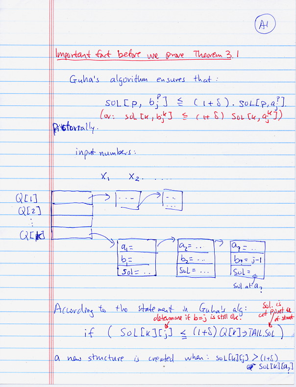
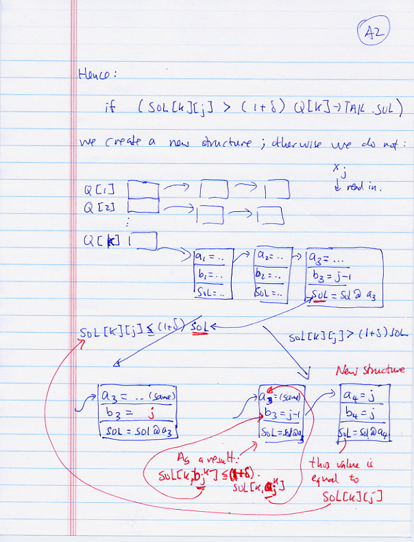
- Algorithm:
  /* ------------------------------------------------
     Help function to compute Error in a bucket
     ------------------------------------------------ */
  SqError(int a, int b)
  {
     s2 = PP[b] - PP[a];
     s1 = P[b] - P[a];
     return (s2 - s1*s1/(b-a+1));
  }

  /* ----------------------------------------------
     Prepare arrays to compute error efficiently
     ---------------------------------------------- */

  P[0] = 0;
  PP[0] = 0;

  for (i = 1; i <= N; i++)
  {
     P[i] = P[i-1] + xi
     PP[i] = PP[i-1] + xi2
  }

  // Note: We don't approximate OPT[1][..]
  //       OPT[1][..] is computed exactly using SqError(a,b)


  /* ------------------------------------------------------------------
     Now we compute the approximate V-opt. histogram with B buckets

     Output:

        BestError[i][k] = best error of histogram
                          using k buckets
			  on data points (1..i)
     ------------------------------------------------------------------ */

  // The dynamic algorithm uses these variables:
  //
  //  k = # buckets
  //  i = current item - items processed are: (1..i)


  // Initialization
  /* -----------------------------------------------------
     Set up (B-1) linked list Q[k] (k = 2..B) to store
     the approximate solution histograms

     Each Q[k] is a linked list of records of the form:

	Q[k].a = left point of bucket
	Q[k].b = right point of bucket
	Q[k].Sol = approximate solution at point Q[k].a
     ----------------------------------------------------- */
  for (k = 2; k <= B; k++)
  {
     Q[k] -> (a = 1, b = 1, Sol = 0);  // List element
  }


  for (k = 1; k <= B; k++)
  {
     // Find optimal histogram using k buckets

     currApprox = Q[k] -> Sol   // initially equal to 0

     for (i = 1; i <= N; i++)
     {
        minError = INFINITE;	 // Start value

       // Try every possible size for the last bucket
        for (j = 1; j <= i-1; j++)	 // Last bucket is [j..i]
        {
           if ( Lookup(Q[k-1], j) + SqError(j+1,i) < minError )
           {
	       minError = Lookup(Q[k-1], j) + SqError(j+1,i);
		                            // Better division found
           }
        }

	if ( minError > (1 + δ) * currApprox )
        {
	   Add new bucket (a = i, b = i, Sol = minError)
	   to Q[k]
	}
     }
  }
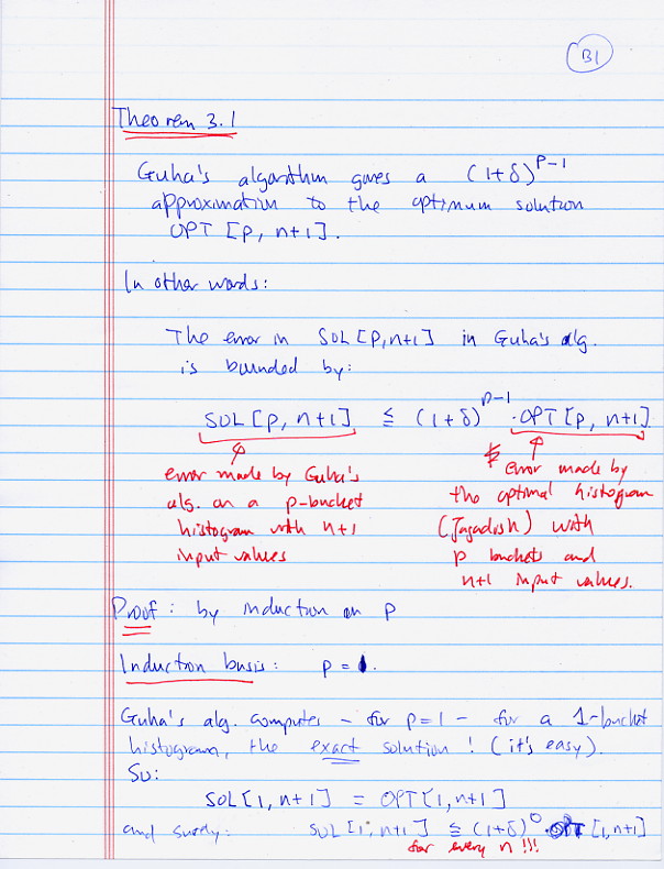
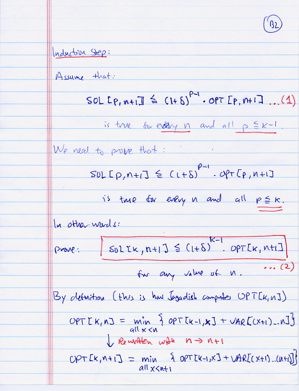
- Theorem 3
of Guha's paper
states:
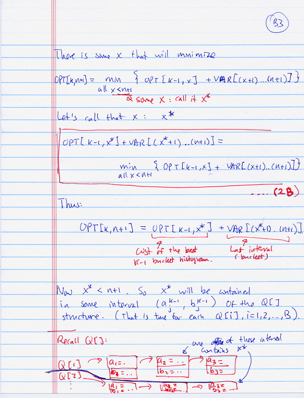
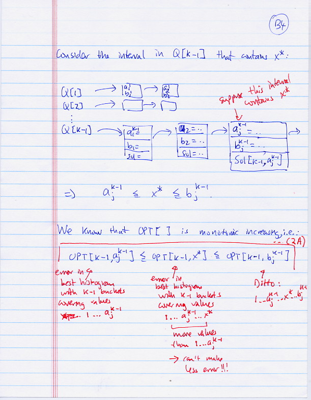
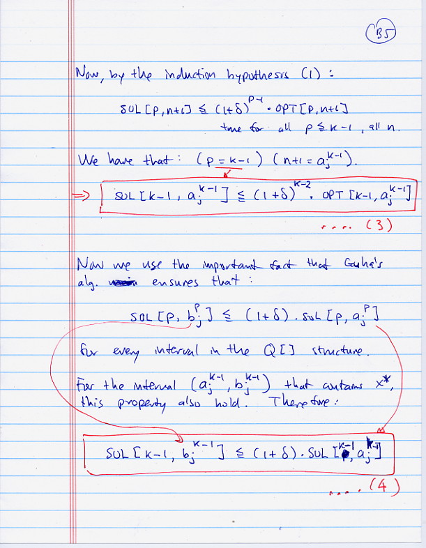
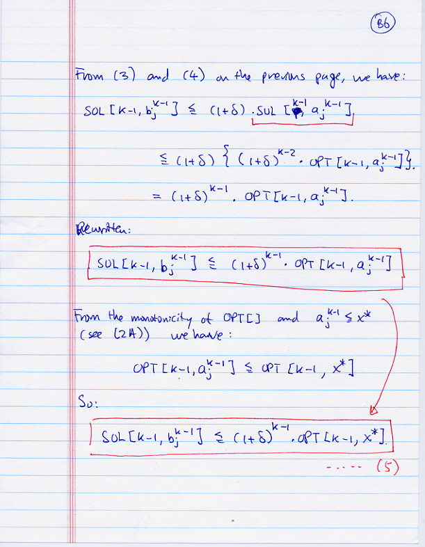
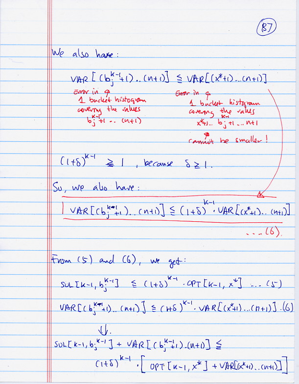
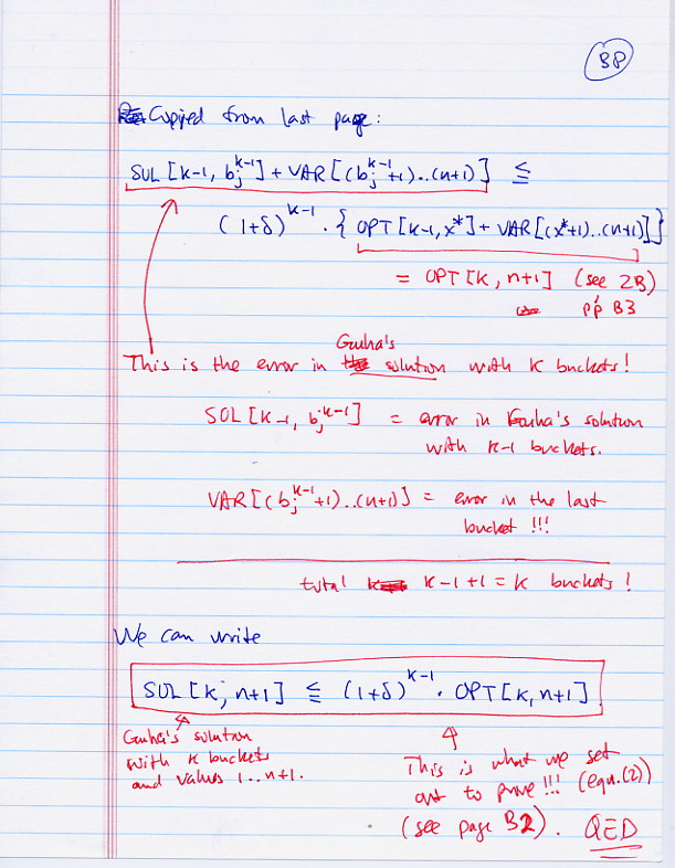
- The algorithm above will compute a histogram with error Sol[p+1,n+1] that is at most (1 + δ)p × OPT[p+1,n+1]
- Proof: (for you eyes only - I retraced the proof...
I will not discuss it in class...)