---

Summary: Queueing Theory and Performance Analysis

---

• Probability (likelihood) of an event
  • The probability of an event A is the likelihood of the occurring of that event.

    Concretely:

    Probability of an event A:

    # outcomes A Ҏ [ event A ] = ------------------------ # posible outcomes

  ---

  ---

• Probability mass/density function (Probability distribution function)
  • The probability mass/density function:

    p(k) = Probab[ event x = k ] I.e.: p(k) = the probability that the outcome x is equal to k (x is called a random variable)

  ---

  ---

• Cumulative probability distribution function
  • Cumulative probability distribution function:

    Discrete p(x): Q(k) = Ҏ[ x ≤ k ] = &sum x ≤ k p(x) Continuous p(x): Q(k) = Ҏ[ x ≤ k ] = &int x ≤ k p(x) Note that: d Q(x) p(x) = ------ dx

    Property of every cumulative probability distribution function:

    lim (x → ∞) Q(x) = 1

  ---

  ---

• Expected value or the mean (average) number of a random variable

  • Mathematical definition of expected value:

    E[x] = ∑(all values k) k Ҏ[k] (discrete x) E[x] = ∫(all values k) x p(x) dx (continuous x)

  ---

  ---

• Conditional Probability

  Conditional Probability Ҏ[A | B]:

  Ҏ[A &cap B] Ҏ[A | B] = ---------- Ҏ[B]

  ---

  ---

• Law of Total Probability (Law of Alternatives or Partitioning Theorem)
  • Law of Total Probability

    Let B1, B2, ... BN finite (or countably infinite) partition of a probability space Then: Ҏ[ A ] = Ҏ[ A | B1 ] × Ҏ[ B1 ] + Ҏ[ A | B2 ] × Ҏ[ B2 ] + ... + Ҏ[ A | BN ] × Ҏ[ BN ]

  ---

  ---

  ---

  ---

• Poisson process
  • The Poisson process is a stochastic event where:

    1. Ҏ[ one customer arrives in the next time interval Δt ] = &lambda×Δt + o(Δt) ........ (1) 2. Ҏ[ no customer arrives in the next time interval Δt ] = 1 - &lambda×Δt + o(Δt) ........ (2) 3. Ҏ[ ≥ 2 customers arrive in the next time interval Δt ] = o(Δt) ........ (3) 4. The arrivals in non-overlapping time intervals are (probabilistically) independent

  ---

  ---

• Poisson (probability) density function
  • Poisson PDF:

    (λT)k Ҏ[ k arrivals in interval of T sec ] = ------- e-λT k!

  ---

  ---

• Expected value (or the mean) of a Poisson λ distributed random variable

  E[x] = λT (avg. # arrivals in interval of T sec)

  ---

  ---

• Arrival rate (# arrivals/sec)
  • Arrival rate:

    Avg # arrivals per second = λT/T = λ

  ---

  ---

• The interarrival times: time between 2 consecutive arrivals in a Poisson process
  • Ҏ[ y ≤ t ] = probability that the inter-arrival time is less that t:

    Ҏ[ y ≤ t ] = 1 - e-λt

  ---

  ---

• Memory-less property of the Poisson arrival process
  • Memoryless property:

    u sec t sec |<---------------->|<-------------------->| Ҏ[ no arrival occurs within next t sec | no arrival for u sec ] = Ҏ[ no arrival occurs within next t sec ]

  • Allows us to compute transition probabilities in Markov chains easily...

  ---

  ---

• Markov chains
  • One-step transition probability:

    Pij = Ҏ[ X(t+1) = j | X(t) = i ]

    ---

  • One-step transition probability matrix:

    +- -+ | P11 P12 P13 ... P1N | | P21 P22 P23 ... P2N | P = | .. .. .. .. | | .. .. .. .. | | PN1 PN2 PN3 ... PNN | +- -+

    ---

  • n-step transition probability matrix:

    Pn = P × P × P × .... × P

    ---

  • Finding the stationary (steady state) state probability π for a Markov chain:

    π = π × P (with: &pi1 + &pi2 + ... + &pin = 1)

  ---

  ---

• Birth-death process: a special Markov process
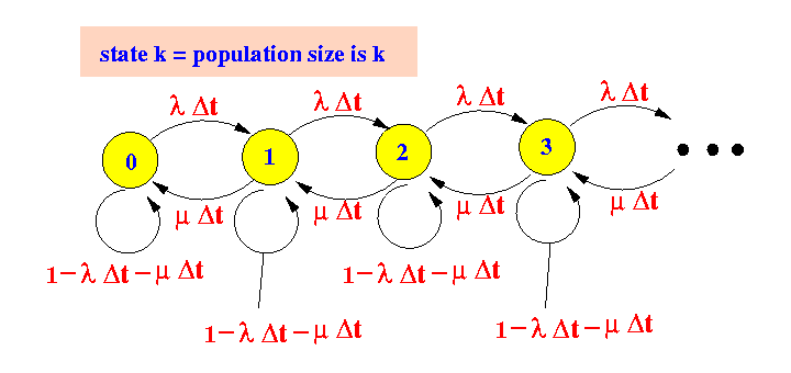
  • Birth-death process only has transitions to its immediate neighbor:

  ---

  ---

• Poission Birth/death process
  • Poisson birth/death process:

    Ҏ[ an arrival occurs in time interval Δt ] = λ × Δt Ҏ[ a departure occurs in time interval Δt ] = μ × Δt λ = arrival rate (see: click here ) μ = departure rate

    ---

    ---

  • State transition diagram for a Poisson birth/death process:

    ---

  • Steady state probability distribution of a Poisson birth/death process with arrival rate λ and departure rate μ:

    p0 = (λ/μ)0 × (1-(λ/μ)) p1 = (λ/μ)1 × (1-(λ/μ)) p2 = (λ/μ)2 × (1-(λ/μ)) p3 = (λ/μ)3 × (1-(λ/μ)) .... Or: p0 = ρ0 × (1 - ρ) p1 = ρ1 × (1 - ρ) p2 = ρ2 × (1 - ρ) p3 = ρ3 × (1 - ρ) .... Or: Ҏ[ k customers in system ] = pk = ρk × (1 - ρ)

  ---

  ---

• M/M/1 Queue: is a Birth/death process
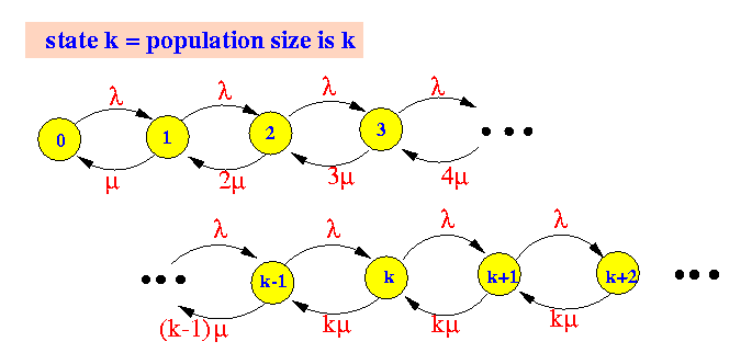
  • The rate transition diagram for the M/M/1 queueing system is:

  ---

  ---

• Other queueing systems
  • The rate transition diagram for the M/M/2 system is:

    ---

  • The rate transition diagram for the M/M/k system is:

    ---

  • The rate transition diagram for the M/M/1/k (finite buffer) queueing system is:

  ---

  ---

  ---

  ---

• Performance analysis
  • Average queue length:

    N = mean (expected) number of customer = 0 × Ҏ[ k customers in system] + 1 × Ҏ[ 1 customer in system] + 2 × Ҏ[ 2 customers in system] + .... = ∑ {k = 0, 1, .., ∞} k × Ҏ[ k customers in system] (definition of "expected value") = ∑ {k = 0, 1, .., ∞} k × pk

    ---

  • Average delay: the Little's formula:

    T = N / λ (Little's formula in another form)